Analyzing the 2025 Board election

“Tyranny of the majority”

I’m sure I’ve shared something like this before, but can’t find it. But it’s easy and important, so bears repeating:

An organization has 500 men and 499 women.

There are 10 open seats.

All 499 women run for election, but only 10 men.

The electorate is absurdly polarized (to make the point clear)::

  • All the men approve of all and only the men.
  • All the women approve of all and only the women.

So each man gets 500 approvals, and each woman 499 approvals.

Under the scheme we’re using now, all 10 seats are filled by men,

Under any scheme making a claim to PR (including, of course, all the ones I sketched here), 5 seats will go to men and 5 to women

This is the kind of example that makes PR “intuitively appealing - even compelling”. But PR is blind to ideology. If, e.g., a quarter of your org consists of closet Nazis, they’ll get about a quarter of the seats too, even if they run openly as such.

9 Likes

Recapping, candidate #10 was our 4th-place finisher, and candidate #6 placed 5th. So #10 made it to the Board, and #6 did not.

Under all versions of PR Approval I tried, their order swapped, and #6 would have made it to the Board instead.

At the start, the top 5 approval-getters were (most to least):

     1 440
    11 439
     8 412
    10 343
     6 328

Under plain Approval, those counts never change, so that shows the final ordering too.

Under h=1 (Jefferson, JS) PR Approval, #1 is picked first, and then ballots are reweighted to reduce the influence of all ballots that approved of #1. This alone swapped the order. Note: I’m showing floats here to make it more obvious. The actual calculations use fractions.Fraction and are exact.

After this reweighting:

    11 293.00
     8 267.50
     6 210.00
    12 199.50
    10 199.00

#10’s standing fell “a lot”, because so many ballots who approved of #10 had already had one of their approvals (#1) win a seat. The overlap between #1 and #6’s supporters was smaller - and of #1 and #12’s (#12 wasn’t even in the top 5 at the start).

And that’s pretty much “the whole” reason for the swap. #11 was picked second, and aftrer reweighting again to reflect that:

     8 184.67
    10 148.33
     6 148.17
    12 140.33
     4 104.17

BIg change! #10 rose above #12 and #6 again, and became nearly tied with #6.

#8 was the 3rd winner, and the reweighting going into the 4th round became:

     6 120.33
    10 120.08
    12 114.42
     4  83.00
     9  56.92

So #6 won, but just barely so.

Under h=2 (Webster, WS), similar, but more pronounced, because it reduces weights faster. Going into its 4th round,

     6  80.27
    10  77.11
    12  75.42
     4  54.17
     9  38.25

#10 was more badly hurt under that by their “association” (in a statistical sense, just staring at correlations among ballots) with the first winner.

2 Likes

And noting that this is one reason for why the .P (“parallel”) versions are preferred. They don’t do “rounds”, but rather score every possible result set on its own, as a whole.

Doesn’t really matter in this election, but can become very clear if there’s ever a tie in a sequential (.S) version’s round. We never had a tie. If there is, the order in which ties are resolved in a sequential version can change the final set of winners, and nobody is happy with that.

Of course parallel versions can tie too, but only among final result sets that score identically. Very unlikely for non-contrived elections. The code I wrote just gives up then.

“Why so cagey? Do you like PR schemes or not?”

It depends on the scheme and/or the context. I can’t be wholly objective about this election because I voted in it.

In general, this form of PR isn’t inherently objectionable to me, I just doubt that adopting it would be a real improvement, because the PSF isn’t yet highly polarized in general. If you read through everything I posted here, “the math” triggered on relatively tiny differences. I couldn’t get outraged over either outcome.

Other forms of PR I do have strong opinions about. In particular, “closed party list PR” seems to me to be a disaster, playing a key role in electing historical (& one current) governments that I consider to be guilty of major crimes against humanity. It tends to elect fractured governing bodies that “have to” cave in to extreme minority demands, from parties so fringe that they could never win a seat without a PR scheme.

But Approval PR has little in common with that scheme beyond the words “proportional representation”. “Closed”, “party”, and “list” all introduce toxic elements that Approval PR has none of.

Clarifying: “the math” is very clear to me, and already explained that today. I know why the switch happened at that microscopic level.

But that’s not the meaning of “why” I had in mind there. What I can’t explain is the social dynamics that drove the math finding the correlations it in fact found. This is about how community members view each other, and I have close to no knowledge of how almost any of the candidates are viewed by others. That’s all about social relations, personal experiences, perceptions of histories, and in-group/out-group distinctions all humans are prone to. Almost everything relevant about the two candidates in question has been invisible to me. Sure, it’s obvious they were well-liked by some, but relatively few of the 683 people who cast ballots spoke up on this forum, and I had no experience of them outside the election topics here.

Deeper insight into that can’t come from me.

In contrast, e.g., I claim I do know “why”, at this higher level, our #12 finisher gets strongly elevated the higher h gets. A whole lot of the social dynamics behind that were extremely visible to everyone on Discourse, and nothing about how PR treated them surprised me at all.

Although I confess they got over twice the approvals I guessed they might get.

More, reducing h to Fraction(94, 100) is enough to make it go away.

And that’s the end of my PR analysis. It (any of the PR methods) would have changed one of those elected to the Board, but just barely. There’s no evidence in these results to be found of systemic disproportional representation of any kind.

1 Like

To be very clear, at this time I would (if anyone asked) recommend not changing to Approval PR (but would recommend switching to Bloc STAR if that goes well for the upcoming SC election).

There isn’t a demonstrated need, and there is, in my judgment, a huge drawback: it ramps up the complexity. One of Approval’s greatest attractions is that it’s the simplest imaginable multi-winner method that “doesn’t absolutely suck” in practice. To the contrary, it works well. I don’t believe anyone is confused by how Approval ballots are scored. “Approve all you like, whoever gets the most approvals wins.” That’s it.

The sequential versions of Approval PR I sketched here are in turn about the simplest PR schemes that exist, but are by any objective measure far more complex. Despite that I’ve long been familiar with them, I spent some hours in all digging into why these schemes acted as they did on our election ballots. In part, that’s my idea of fun :wink:, but I don’t wish it on anyone else.

In short, ain’t broke, don’t fix.

4 Likes

Just for fun, for those inclined, take a stab at implementing “Satisfaction Approval Voting”. You can find mountains of info on the web. Not a method I recommend, but it’s a way to learn things in a relatively simple extension of Approval.

The goal here is to pick a set of winners that maximizes “total voter satisfaction”, where the satisfaction of a voter is the number of winners they got divided by the number of approvals they made. So if everyone they approved of won, their “satisfaction” is 1.0. If none won, 0.0. If half won, 0.5. And so on. Ignore empty ballots.

You’re looking for a set of winners that maximizes the sum of all voters’ satisfactions.

It’s not a PR scheme, but “semi-proportional”. Look on the web for involved explanations of the distinctions.

But it’s intuitively clear. Note in particular that it’s inherently “parallel” in the sense I introduced in this topic: you have to know the full set of winners in order to score. There is no “sequential” way here to pick one winner at a time. It’s expensive (technically, in the class NP-hard) to compute.

You can’t do much better than generate all possible sets of winners, and score each on its own. In that respect, it’s like JP and WP here. But that also makes the code short and straightforward to write (hint: itertools.combinations)..

Cute: on our ballots, it too uniquely picks the same 4 winners picked by our JS, WS, JP, and WP.

1 Like

Unsurprisingly, all 5 didn’t approve of the same candidate. One guess as to which :wink:.

Somewhat surprisingly, of the 5 “anyone but two” ballots, two of these did approve of that candidate. Across them, 7 distinct candidates didn’t get approved, 5 of those excluded by only one of the ballots.

And here’s a 13x13 correlation matrix. a[i, j] (1-based indices) gives the correlation between candidates #i and #j, and is symmetric (a[j, i] is the same).

  • This is “the standard” Pearson correlation coefficient, but multiplied by 100 and rounded to an int,.to cut the amount of horizontal space needed for display.

  • It’s mathematically constrained to be between -100 and 100 inclusive. 100 is perfect correlation: every ballot either approves of both or of neither. -100 is perfect anti-correlation: no ballot approves of both.

  • Negative correlations are rare in our data, in large part because we have a pile of ballots that approved of everyone.

  • I was surprised that we have no correlations reaching 50;. There are simply no strong correlations between any candidate pair.

  • From a PR view, one of the strongest correlations (41) is between candidates #1 and #10. Which is why PR schemes hammered #10’s chances when #1 was picked as the first winner. The correlation between #1 and #6 is much weaker (15), so picking #1 did little harm to #6’s chances (who went on to win a seat under all the PR schemes tried).

  • Another of the stronger correlations is between our two bottom-place finishers. To my eyes, they have nothing much in common, except that they’re almost certainly both viewed as “non-mainstream outsiders”. Which suggests there’s some cohort voting for “I don’t really care who, I just want change”.

  • Cute from a technical view: the PR schemes don’t “compute correlations” at all, and their math is actually simpler than the code used to produce this table. The PR code doesn’t have to know anything about correlations to pick up on their effects. They’re quite magical that way :smile:,

    j  1   2   3   4   5   6   7   8   9  10  11  12  13
  i +---------------------------------------------------
  1 |  ,  20  -3  26  13  15   0  15  21  41   6  24   7 
  2 | 20   ,  31  28  39  14  26  12  42  25   2  14  29 
  3 | -3  31   ,   9  33  15  35  10  29  10  10  11  27 
  4 | 26  28   9   ,  34  17  11  20  30  21  16  20  30 
  5 |  3  39  33  34   ,  13  37   8  41  22   6  13  45 
  6 | 15  14  15  17  13   ,   6  14  20  21  16  12  12 
  7 |  0  26  35  11  37   6   ,   5  24   4   3   2  28 
  8 | 15  12  10  20   8  14   5   ,   8  13  33  16  12 
  9 | 21  42  29  30  41  20  24   8   ,  31   1  22  33 
 10 | 41  25  10  21  22  21   4  13  31   ,   7  13  12 
 11 |  6   2  10  16   6  16   3  33   1   7   ,  20   5 
 12 | 24  14  11  20  13  12   2  16  22  13  20   ,  19 
 13 |  7  29  27  30  45  12  28  12  33  12   5  19   , 
1 Like

And here’s a 13x13 conditional probability matrix, a different way to view correlations.. Easiest to understand by columns. a[i, j] (1-based indices) answers this question::given that a ballot approved of candidate #j, what’s the probability that it also approved of candidate #i? This is not necessarily symmetric.

The strongest connection here is that 84% of the ballots approving candidate #10 also approved candidate #1. Another slant on why PR schemes are reluctant to let them both win.

    j  1   2   3   4   5   6   7   8   9  10  11  12  13
  i +---------------------------------------------------
  1 |  .  82  62  81  83  72  65  70  83  84  67  76  73 
  2 | 30   .  51  40  71  30  54  27  56  34  24  30  53 
  3 | 18  41   .  24  56  25  57  22  40  23  22  24  45 
  4 | 45  60  45   .  81  44  49  43  62  45  41  46  70 
  5 | 14  33  32  25   .  15  43  13  35  18  12  15  45 
  6 | 54  61  63  60  67   .  57  54  66  58  54  54  62 
  7 | 12  27  35  16  45  14   .  13  26  13  12  12  33 
  8 | 66  71  71  74  72  67  67   .  68  67  72  69  75 
  9 | 30  54  48  40  72  31  51  26   .  36  23  33  56 
 10 | 65  73  61  64  81  61  56  56  79   .  53  57  65 
 11 | 66  66  74  74  72  72  68  77  65  68   .  75  70 
 12 | 56  60  58  61  65  54  49  54  67  54  55   .  70 
 13 | 17  33  35  29  60  19  42  18  36  19  16  22   . 
1 Like

And putting to rest another minor mystery about the PR results: after the first winner was picked, #10 fell “a lot”, and #6 overtook them. But after the next two were picked, #10 almost managed to regain their lead. Why?

Turns out the next 2 winners picked were the two incumbents, and we had 79 ballots approving of those two and #6 So that in turn hammered #6’s chances.

Another reason for why the “.P” versions are easier to live with (despite being more costly to compute):: things can thrash back and forth doing things “one at a time”, and burn a lot time figuring out “why”. The “.P” versions skip straight to the final score, and there is no thrashing to unwind.

Clustering.

Another line of analysis is quantifying “how similar” ballots are. There were 2^{13} possible distinct ways to fill out a ballot in this election, but despite that we had only 683 ballots (which could cover no more than 9% of the possibilities), they were hardly all unique. They “clump”.

So how “similar” are two ballots? Given sets (of approvals, here) S and T, Hamming distance is a popular measure: len(S ^ T). It counts how many elements appear in only one. The smaller, the more similar. and 0 if and only if S == T.

But that’s unsatisfying in this context because it doesn’t take the size of the sets into account. {1} and {1, 2} have Hamming distance 1, same as {1,2,3,4,5,6,7,8} and {1,2,3,4,6,7,8}, but the latter pair is obviously “much more similar” than the former to human eyes.

“Jaccard similarity” is more on target: a float in 0.0 (the sets have nothing in common) to 1.0 (the sets are the same). If S and T are both empty, it’s 1.0. Else it’s len(S & T) / len(S | T), the number of elements in common divided by the number of distinct elements total. {1} and {1, 2} have similarity 1/2 by this measure, while{1,2,3,4,5,6,7,8} and {1,2,3,4,6,7,8} have similarity 7/8. Better.

Next, given a measure, how can we use it to group ballots into similar cluslters? There is no definitive answer to that. Consider a simpler context, grouping the ints 3, 4, 5 into maximal sets whose elements are “within 1” of each other. [{3, 4}, {5}] and [{3}, {4, 5}] both work for that. There just isn’t a unique grouping.

I use a common compromise. Start with an empty list of “equivalence classes” (an abuse of terminology, but helpful in context). Given a similarity floor minsim, the next ballot marches over that list, and adds the ballot to the first class found (if any) where every element in the class is at least within minsim of the new ballot. If no such class is found, the new ballot is added as a new singleton equivalence class.

So, a lot of preliminaries.

First thing to try is similarity 0. This puts all ballots into the same class:

Jaccard similarity 0 yields 1 equivalence class
    1 class with 683 ballots each

Next is to try similarity 1. This breaks the ballots into classes each of which contains identical ballots. Output is ordered by deceasing cardinality of equivalence class:

Jaccard similarity 1 yields 338 equivalence classes
    1 class with 23 ballots each
    1 class with 15 ballots each
    2 classes with 14 ballots each
    2 classes with 11 ballots each
    1 class with 10 ballots each
    4 classes with 9 ballots each
    7 classes with 8 ballots each
    3 classes with 7 ballots each
    2 classes with 6 ballots each
    9 classes with 5 ballots each
    9 classes with 4 ballots each
    17 classes with 3 ballots each
    48 classes with 2 ballots each
    232 classes with 1 ballot each

So we had only 338 distinct ballots. The most populated class contained 23 ballots, which was identified before as the “I approve of everyone” ballot.

It’s at least “interesting”, e.g., that there were groups of 8 identical ballots, and that was so 7 times. The voters casting those ballots viewed the candidates the same way, However, the largest equivalence class had only 23 members, and in a situation where PR would make a major difference, the electorate would show much more duplication.

Coordinated gamers would try to “hide” their games by not casting identical ballots, but things don’t change all that much if the similarity threshold is cut to 80%:

Jaccard similarity 0.8 yields 265 equivalence classes
    1 class with 31 ballots each
    1 class with 17 ballots each
    2 classes with 16 ballots each
    1 class with 15 ballots each
    3 classes with 14 ballots each
    1 class with 12 ballots each
    2 classes with 11 ballots each
    3 classes with 10 ballots each
    2 classes with 9 ballots each
    4 classes with 8 ballots each
    2 classes with 7 ballots each
    4 classes with 6 ballots each
    6 classes with 5 ballots each
    11 classes with 4 ballots each
    22 classes with 3 ballots each
    54 classes with 2 ballots each
    146 classes with 1 ballot each

There are numerous small groups of voters who voted much the same way, but PR aims to elevate small groups by kneecapping large groups, and there are no large sufficiently like-minded groups in sight.

In the limit, each voter is a minority of 1, and they can’t all win :wink:,.

1 Like

The 2nd-highest number of duplicate ballots (15) didn’t stick out via any prior form of digging into the data. What’s up with that? This is 15 copies of a 4-approval ballot. They approved of our top 3 vote getters, and one other (#X) who did quite well, but below the 4-winner cutoff.

Jefferson PR would not have helped them, but the more aggressive Webster PR would have boosted them, by one position. However, as I alluded to before, if “the rules” change, so would voter behavior. Under the likely (to me) belief that most of these duplicated ballots came from real-life friends who discussed 'the best way" to vote [1], under PR they could well have figured out that approving the incumbents (who were likely to win regardless) too would only hurt #X’s chances. As is, when it came to the 4th round, under Webster these ballots only carried 1/7th of their original weight, so these 15 ballots would only add 15/7 to #X’s score. #X’s chances would have been materially improved if they had not approved of the incumbents.

But that’s under PR, which opens ways for trying to game the system that don’t exist in plain Approval.


  1. nothing wrong with that! ↩︎

Voter similarity,.

I’m trying to advance the state of the art here - so take this with a grain of salt. I don’t think you’ll find this one in the literature.

How much alike are candidate #i and candidate #j’s voters? Of course all we know about them is how they voted.

In outline:

initialize an empty Counter for each candidate
for each ballot:
    for each candidate approved by that ballot:
        update that candidate's Counter with the entire ballot

Now, for each candidate, we have a multiset of all the approvals that candidate’s voters made. How similar two candidates’ voters are is taken to be how similar their multisets are. This is a symmetric measure.

Problem: different candidates attract different numbers of approvals, so these multisets can have very different cardinalities (which is given by Counter.total(), not by led(Counter)). So … we scale them to have the same cardinalities. For each multiset C, we multiply C’s counts by L // C.total(), where L is the math.lcm() of all the multisets’ cardinalities.

Now we’re golden. the obvious generalization of Jaccard similarity is used to compute multisets’ similarity (same formula, but using .total() instead of len()).

As usual, the results here are multiplied by 100 and rounded to int, to keep lines short.

The values span a surprisingly small range. As a sanity check, it’s no surprise that the single “most similar” candidates’ voters are those who approved of the two incumbents, with score 89. The least similar were the voters for the incumbents and those who voted for He Who Will Romain Nameless - but even those scores are close to 60.

Cute; the lcm of the multisets’ cardinalities turned out to be

899_610_003_014_102_747_852_879_870_636_160

I am soooooooooo glad I did this in Python :smiley:,

    j  1   2   3   4   5   6   7   8   9  10  11  12  13
  i +---------------------------------------------------
  1 |  .  71  67  80  62  83  60  83  72  87  82  84  66 
  2 | 71   .  78  77  78  72  75  70  86  73  69  72  80 
  3 | 67  78   .  73  75  68  79  67  77  70  65  68  78 
  4 | 80  77  73   .  69  80  66  79  77  82  77  81  73 
  5 | 62  78  75  69   .  63  78  61  78  64  60  63  82 
  6 | 83  72  68  80  63   .  62  84  73  83  83  83  67 
  7 | 60  75  79  66  78  62   .  60  73  63  59  62  78 
  8 | 83  70  67  79  61  84  60   .  71  81  89  84  66 
  9 | 72  86  77  77  78  73  73  71   .  74  69  72  80 
 10 | 87  73  70  82  64  83  63  81  74   .  79  82  68 
 11 | 82  69  65  77  60  83  59  89  69  79   .  83  64 
 12 | 84  72  68  81  63  83  62  84  72  82  83   .  67 
 13 | 66  80  78  73  82  67  78  66  80  68  64  67   . 

This isn’t satisfying, but for now I lack a better idea. As noted when I mentioned Hamming distance, “a problem” with that is that it doesn’t take set size into account. Jaccard does, but that backfires some when generalized to multisets.

If A’s voters gave A 100 approvals and also to B, and B’s voters gave 10 to each, are they really different? The normalization I sketched above multiplies the counts in B’s multiset by lcm(200, 20) // 20 == 10, and A’s counts by 1, making them appear identical. Without that, Jaccard similarity would have been 20/200 = 0.1. Which is all the raw data actually justifies. Scaling expediently assumes that if a candidate had gotten more approvals, the fantasy ballots would reproduce the same relative distribution across all candidates.

I’ll show results if scaling is skipped. There’s a much larger spread of scores then, but many of them are really just reflecting that, e.g, candidate #5 got a lot fewer approvals than #1. When sets are of different size, an upper bound on Jaccard similarity is the cardinality of the smaller divided by the cardinality of the larger.

    j  1   2   3   4   5   6   7   8   9  10  11  12  13
  i +---------------------------------------------------
  1 |  .  47  35  63  27  72  22  82  47  80  82  73  31 
  2 | 47   .  69  66  54  56  45  49  86  54  47  56  61 
  3 | 35  69   .  50  67  45  57  38  68  41  37  44  73 
  4 | 63  66  50   .  41  74  33  66  67  71  64  75  46 
  5 | 27  54  67  41   .  33  74  28  54  32  28  33  78 
  6 | 72  56  45  74  33   .  28  76  57  82  75  83  39 
  7 | 22  45  57  33  74  28   .  24  44  26  23  28  64 
  8 | 82  49  38  66  28  76  24   .  49  79  89  76  33 
  9 | 47  86  68  67  54  57  44  49   .  55  47  57  61 
 10 | 80  54  41  71  32  82  26  79  55   .  77  80  36 
 11 | 82  47  37  64  28  75  23  89  47  77   .  75  32 
 12 | 73  56  44  75  33  83  28  76  57  80  75   .  39 
 13 | 31  61  73  46  78  39  64  33  61  36  32  39   . 

An AI chatbot suggested I look into using “cosine similarity” for this. Duh! Great idea I just overlooked. It measures “closeness” not by magnitude or overlap, but by the (cosine of the) angle between multisets (represented by 13-dimensional vectors).

Promising idea, and no rescaling needed. Alas, it appears to suck :frowning:. Now the scores are unhelpfully “too large” in an even narrower range. I think “the problem” boils down to that the “angles” are dominated by the axes containing the top overall vote-getters, and those show up in all multisets. So all pairs “look pretty close”. Exacerbated by that the cosine function has a zero derivative at angle 0 (changes slowly across angles near 0).

    j  1   2   3   4   5   6   7   8   9  10  11  12  13
  i +---------------------------------------------------
  1 |  .  93  88  96  88  96  85  97  93  98  96  96  89 
  2 | 93   .  93  94  95  91  91  91  96  93  90  91  93 
  3 | 88  93   .  89  93  90  93  89  92  89  89  89  92 
  4 | 96  94  89   .  92  94  87  95  94  95  94  94  93 
  5 | 88  95  93  92   .  87  93  86  95  89  86  87  96 
  6 | 96  91  90  94  87   .  85  95  92  95  96  94  89 
  7 | 85  91  93  87  93  85   .  85  90  85  85  84  91 
  8 | 97  91  89  95  86  95  85   .  90  95  98  96  89 
  9 | 93  96  92  94  95  92  90  90   .  94  89  92  94 
 10 | 98  93  89  95  89  95  85  95  94   .  95  95  89 
 11 | 96  90  89  94  86  96  85  98  89  95   .  96  88 
 12 | 96  91  89  94  87  94  84  96  92  95  96   .  90 
 13 | 89  93  92  93  96  89  91  89  94  89  88  90   . 

This “voter similarity” is getting somewhere now - and intriguingly so. After much thought, it dawned on me that cosine similarity views vectors (multisets) as rooted at the all-0 origin in 13D space. Since each vector’s components are all positive, it can’t find an angle outside the range 0-90 (degrees).

Instead it “should” view the origin as being at the multisets’ centroid (for each component, the mean of all the multisets’ corresponding component). Then it “suddenly” becomes sensitive to whether a multiset’s voters are giving candidates more, or less, approvals than average. Such differences now don’t just tweak the angle a little, they can give an angle of a different sign (the voters are giving approvals in opposite directions from “average”)..

Then things get interesting indeed. Now results are all over the place, in the range -100 to 100. This is just cosine similarity again, but tweaked to subtract the multisets’ centroid from each multiset first. So they no longer represent absolute counts, but instead signed differences from the average.

Each candidates’ voters can look very different under this measure.

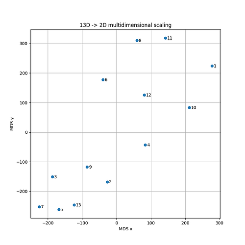
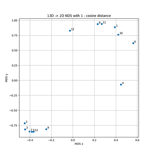
But still keep that grain of salt! I’m “pioneering” here, and am not even sure the code doesn’t have crucial bugs. Still, this makes good quantitative sense of several patterns I noticed by eyeball (for example, #7 and #5’s voters appeared to vote very much like, but #7 and #1’s voters very much unalike), but just don’t stand out under any other line of analysis I’ve tried. Here, they punch you in the nose :wink:.

    j  1   2   3   4   5   6   7   8   9  10  11  12  13
  i +---------------------------------------------------
  1 |  . -79 -93  14 -93  62 -93  80 -79  84  79  67 -93 
  2 |-79   .  81  -9  85 -67  82 -83  82 -66 -86 -69  82 
  3 |-93  81   . -25  93 -65  94 -84  80 -80 -83 -70  91 
  4 | 14  -9 -25   . -12  -2 -19   8  -9   5   6   3 -11 
  5 |-93  85  93 -12   . -72  98 -91  86 -80 -91 -73  97 
  6 | 62 -67 -65  -2 -72   . -70  60 -64  55  64  42 -72 
  7 |-93  82  94 -19  98 -70   . -88  82 -82 -88 -73  96 
  8 | 80 -83 -84   8 -91  60 -88   . -86  65  89  62 -88 
  9 |-79  82  80  -9  86 -64  82 -86   . -63 -88 -64  83 
 10 | 84 -66 -80   5 -80  55 -82  65 -63   .  63  48 -82 
 11 | 79 -86 -83   6 -91  64 -88  89 -88  63   .  67 -89 
 12 | 67 -69 -70   3 -73  42 -73  62 -64  48  67   . -69 
 13 |-93  82  91 -11  97 -72  96 -88  83 -82 -89 -69   .