Dear all,
I am working on an astronomy project, but to explain in relevant and layman’s terms, I am attempting to fit data, calculated from an equation using four parameters as open parameters, to observed data in order to calculate a realistic value for one of the open parameters. For the open parameters, I used a grid search based approach to iterate over initial values within the bounds of what is physically possible for the parameters. Here is the simplest version of my code:
import numpy as np
import matplotlib.pyplot as plt
from scipy.optimize import curve_fit
import pygyre as pg

delta_pg = 125
delta_nu = 32

# Function to extract frequencies and radial orders from the summary file
def read_frequencies_and_orders(summary_file):
    s = pg.read_output(summary_file)
    l_values = s['l']  # Angular degree
    n_pg_values = s['n_pg']  # Radial order
    freq_values = s['freq'].real  # Frequencies in micro Hertz
    return l_values, n_pg_values, freq_values

# Read the frequencies and radial orders from the summary file
summary_file = 'summary.h5'
l_values, n_pg_values, nu_values = read_frequencies_and_orders(summary_file)

# Filter to only include l=1 modes
l1_indices = np.where(l_values == 1)[0]
n_values = n_pg_values[l1_indices]
nu_values_l1 = nu_values[l1_indices]

# Filter to include l=0 modes for calculating the uncoupled p-mode frequencies
l0_indices = np.where(l_values == 0)[0]
nu_values_l0 = nu_values[l0_indices]

# Calculate uncoupled p-mode frequencies as the midpoint between consecutive l=0 modes
nu_np_l1 = []
for i in range(len(nu_values_l0) - 1):
    mid_point = (nu_values_l0[i] + nu_values_l0[i + 1]) / 2
    nu_np_l1.append(mid_point)
nu_np_l1 = np.array(nu_np_l1)

# Truncate nu_values_l1 to match the length of nu_np_l1
nu_values_l1 = nu_values_l1[:len(nu_np_l1)]

# Asymptotic relation for mixed modes with flexible delta_pg and delta_nu
def mixed_mode_relation(nu, epsilon_g, q, delta_pg_flex, delta_nu_flex):
    term1 = np.pi * (1 / (delta_pg_flex * nu) - epsilon_g)
    return nu_np_l1 + (delta_nu_flex / np.pi) * np.arctan(q * np.tan(term1))

# Perform a grid search over possible values of q and epsilon
q_grid = np.linspace(0.000001, 1, 100)  # grid for q
epsilon_grid = np.linspace(0.00001, 1, 100)  # grid for epsilon

# Define a function to calculate residuals
def calculate_residuals(nu_values, epsilon, q):
    predicted_nu = mixed_mode_relation(nu_values, epsilon, q, delta_pg, delta_nu)
    return np.sum((nu_values - predicted_nu) ** 2)

# Perform grid search
best_q = 0
best_epsilon = 0
min_residuals = float('inf')

for epsilon in epsilon_grid:
    for q in q_grid:
        residuals = calculate_residuals(nu_values_l1, epsilon, q)
        if residuals < min_residuals:
            min_residuals = residuals
            best_q = q
            best_epsilon = epsilon

print(f'Grid Search Results: Best q = {best_q}, Best epsilon = {best_epsilon}')

# Bounds for delta_pg and delta_nu to allow small flexibility
delta_pg_bounds = [delta_pg * 0.95, delta_pg * 1.05]
delta_nu_bounds = [delta_nu * 0.95, delta_nu * 1.05]

# Use least-squares fitting to refine the estimates with flexible delta_pg and delta_nu
popt, pcov = curve_fit(
    lambda nu, epsilon, q, delta_pg_flex, delta_nu_flex: mixed_mode_relation(nu, epsilon, q, delta_pg_flex, delta_nu_flex),
    nu_values_l1,
    nu_values_l1,
    p0=[best_epsilon, best_q, delta_pg, delta_nu],
    bounds=([0, 0, delta_pg_bounds[0], delta_nu_bounds[0]], [np.inf, 1.0, delta_pg_bounds[1], delta_nu_bounds[1]])
)

epsilon_fit, q_fit, delta_pg_fit, delta_nu_fit = popt

# Print the fitted parameters
print(f"Fitted epsilon: {epsilon_fit}")
print(f"Fitted q: {q_fit}")
print(f"Fitted delta_pg: {delta_pg_fit}")
print(f"Fitted delta_nu: {delta_nu_fit}")

# Calculate the fitted frequencies
nu_fitted = mixed_mode_relation(nu_values_l1, epsilon_fit, q_fit, delta_pg_fit, delta_nu_fit)

# Plot the observed and fitted frequencies
plt.figure(figsize=(10, 6))
plt.plot(nu_values_l1, nu_values_l1, 'bo', label='Observed Frequencies')
plt.plot(nu_values_l1, nu_fitted, 'r+', label=f'Fitted Frequencies, q = {q_fit:.4f}')
plt.xlabel('Frequency (micro Hz)')
plt.ylabel('Frequency (micro Hz)')
plt.title('Observed vs Fitted Frequencies for l=1 Modes')
plt.legend()
plt.show()
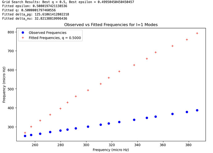
However, the fitted values (red) have huge discrepancies with the observed values (blue), and my q value is off from where I expect (0 - 0.5):
When I change my q bounds to (0 - 0.5), I get this error:
ValueError: `x0` is infeasible.
Assuming all the astrophysics is correct, is there perhaps a better way to calculate the fitting besides scipy.curve_fit?


