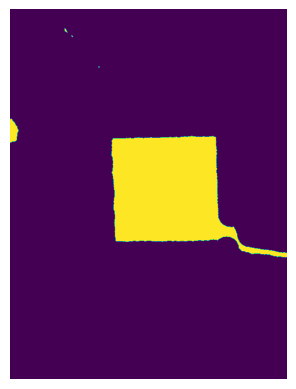
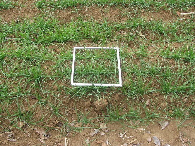
How can I detect and crop the rectangular frame in the image?

[Haqueshenas (Abbas Haghshenas)]

Hi,

I have an archive of images taken from a green field, with a quadrat (i.e. a white rectangular frame) almost in the center of each image. I need to open the images from Input folder, crop the inner part of the quadrate, and save the image in the Output folder, without any change in other image properties (i.e. without interpolation, color normalization, etc.). It is notable that the images have been taken from different heights. Is it possible to do that automatically, or the task should be user-supervised?

[petersuter]

For classic image segmentation techniques try skimage.

It has things like:

• edge detection filters (sobel, canny, …)
• line detection transform (hough)
• corner detection (harris)

But if the colors are so distinct as in your example, you could also try simple color space transform (HSV), thresholding, morphological operations (opening, closing), and filling the rectangle with component labeling:

import skimage.color
import skimage.io
import skimage.measure
import skimage.morphology
import numpy

image_rgb = skimage.io.imread("file.jpeg")

image_hsv = skimage.color.rgb2hsv(image_rgb)
seg = image_hsv[:,:,1] < 0.10

seg_cleaned = skimage.morphology.isotropic_opening(seg, 1)
seg_cleaned = skimage.morphology.isotropic_closing(seg_cleaned, 25)

def get_main_component(segments):
    labels = skimage.measure.label(segments)
    if labels.max() == 0:
        return segments
    return labels == numpy.argmax(numpy.bincount(labels.flat)[1:]) + 1

background = get_main_component(~seg_cleaned)
filled = ~background 

mask = skimage.morphology.isotropic_opening(filled, 25)

masked_result = image_rgb.copy()
masked_result[~mask,:] = 0

mask_x = mask.max(axis=0)
mask_y = mask.max(axis=1)
indices_x = mask_x.nonzero()[0]
indices_y = mask_y.nonzero()[0]
minx, maxx = int(indices_x[0]), int(indices_x[-1])
miny, maxy = int(indices_y[0]), int(indices_y[-1])

cropped_result = image_rgb[miny:maxy, minx:maxx, :]

For different heights and condition you might have to adjust the various parameters.

A more advanced approach would be machine learning convolutional networks.

[Haqueshenas (Abbas Haghshenas)]

Thank you very much for the code and also the valuable description. I got the story.
However, as a beginner, I could not take the results as the same as your run. Could you please help me to find the mistake? I tried to re-run the code and save the image using the below line:
cropped_result = image_rgb[miny:maxy, minx:maxx, :]
cv2.imwrite(“res.JPG”,cropped_result)

This is my result:

[petersuter]

The color change is probably because cv2 assumes BGR colors.
Maybe try cv2.imwrite('res.JPG', cv2.cvtColor(cropped_result, cv2.COLOR_RGB2BGR)) instead.
(More information)

To figure out why you get different cropping, try saving after each step to check at which step it goes wrong.

[Haqueshenas (Abbas Haghshenas)]

The problem was solved by changing the value in the below line from 25 to 80 or 100:

mask = skimage.morphology.isotropic_opening(filled, 25)

I am not sure about the reason; however, I found out that when I copy the image into the code folder (in PyCharm) before running, it is saved with 90 degrees rotation. Also, this is the case when I use windows image viewer.

Thanks a lot.

[petersuter]

It could be that I saved only a small preview instead of the full image. Maybe that explains why the value 25 worked for me.

[Haqueshenas (Abbas Haghshenas)]

I found out that the resolution of the output images are reduced. What is the reason and how can I solve the problem?
Besides, is there any method to check the possible changes in color quality, resolution, and any other unwanted feature of the images?

[petersuter]

@Haqueshenas

the resolution of the output images are reduced

The output images are cropped (fewer total pixels) but the resolution (pixels per area) is the same. The pixels / color quality / resolution in the cropped area are 100% identical to the input image.

[Haqueshenas (Abbas Haghshenas)]

Thanks. Indeed, the properties of a sample input image is as below:
Dimension: 3264*2448
Resolution: 180 dpi
Depth: 24 Bit
Size: 6.16 MB

However, after processing (either segmentation, or cropping in the next level), the resolution of the image is reduced to 96 dpi. The output image will be represented in the next comment.

[Haqueshenas (Abbas Haghshenas)]

The output image (saved after segmentation):

[petersuter]

@Haqueshenas

Dimension: 3264*2448
Resolution: 180 dpi
Depth: 24 Bit
Size: 6.16 MB

(If I download it from here it is smaller. Maybe it gets resized by the server discussion software.)

So the dimensions of the result are the same, right?
180 dpi is additional metadata, separate from the image pixels itself. It’s almost always set to 96 dpi by default. You would have to use a low level image IO library like pillow to read / write dpi metadata explicitly.

[kknechtel (Karl Knechtel)]

Instead of looking at the resolution that an image editor reports for the image, check how many pixels across and down it is for the square in each image.

[Haqueshenas (Abbas Haghshenas)]

This approach was so useful. However, processing a relatively huge image archive, I found some exceptions which need more processing. For instance, this is the result of segmentation of an image in which an unwanted patch has been left at the right bottom corner of the image. I tried to remove it using the “skimage.segmentation.clear_border” command; however it did not work. How can I remove such areas from anywhere on the image boundary?

Thanks

[petersuter]

skimage.segmentation.clear_border seems to work on that image here:

Input mask: (input_mask = skimage.color.rgb2gray(image_rgb) > 0)

Output mask: (output_mask = skimage.segmentation.clear_border(input_mask))

[Haqueshenas (Abbas Haghshenas)]

@petersuter

output_mask = skimage.segmentation.clear_border(input_mask)

Thank you. I had used it in a wrong place in the code.

[petersuter]

(I’m curious, is the dataset / archive of images public? Can you reveal a bit about the context / goal / background of this project and what field it is related to? Just out of interest. )

[Haqueshenas (Abbas Haghshenas)]

Thank you for your consideration. The context is the multidisciplinary and newly emerged area of “Modern crop phenotyping”. Among the subfields of this area are “image-based phenotyping” and “ground-based imaging”, which aims to determine the phenotype (or visible status) of crop canopies (or plants) more rapidly, efficiently, precisely, and also quantitatively.

The purpose of the present project (our project) is to evaluate the effect of several variables (i.e. sensor/camera, height, and imaging time) on the output of the recently introduced model of GSM (green-gradient based canopy segmentation model), which provides a new definition of green canopy based on the shading patterns. Of course, as many other measurements in crop science, sampling is a basic and important practice, which is carried out here, using a white framework (quadrat); particularly if the canopy is not uniform, or parts of other unwanted experimental plots have been taken in the image.
Here, I have several hundred images, which should be pre-processed (i.e. cropped) before used as the inputs of GSM model.
Currently, the archive is not public, but I can send you some more images. Moreover, there are public archives of various crop species available on the internet.
In general, modern crop phenotyping faces various topics and questions to be addressed using image processing. In this context, you can find many studies, codes, and tools on processing of ground based images of experimental plots grown in the field, 3D reconstruction of single plant, plant root system 3D reconstruction (mostly using CT-scan or MRI images) and respective measurements, seed and grain processing, etc. However, compared with the potential of contribution of the data stored in the images, it seems that there is still more work to be done in image processing techniques for modern crop phenotyping.
Obviously, as a researcher in crop science, I prefer to use ready tools; however, they are not available enough and I should write my own codes as a beginner in image processing and coding. Considering the relative novelty of this field, even very simple codes and tools of image processing may lead to considerable findings and achievements in crop science and plant breeding. Only for instance, you can find such simplicity and applications in our publications:

Haghshenas, A., & Emam, Y. (2019). Image-based tracking of ripening in wheat cultivar mixtures: A quantifying approach parallel to the conventional phenology. Computers and Electronics in Agriculture, 156, 318-333.

Haghshenas, A., & Emam, Y. (2019). Evidence for relative grain yield simulation by red color level of beneath-canopy soil at wheat booting phase: An unexpected observation using image processing. Computers and Electronics in Agriculture, 162, 1028-1034. doi:https:/ /doi.org/10.1016/j.compag.2019.05.044

Haghshenas, A., & Emam, Y. (2020). Green-gradient based canopy segmentation: A multipurpose image mining model with potential use in crop phenotyping and canopy studies. Computers and Electronics in Agriculture, 178, 105740. doi:https:/ /doi.org/10.1016/j.compag.2020.105740

Haghshenas, A., Emam, Y., Sepaskhah, A. R., & Edalat, M. (2021). Can extended phenology in wheat cultivar mixtures mitigate post-anthesis water stress? European Journal of Agronomy, 122, 126188. doi:https:/ /doi.org/10.1016/j.eja.2020.126188

Haghshenas, A., Emam, Y., & Jafarizadeh, S. (2022). Wheat grain width: a clue for re-exploring visual indicators of grain weight. Plant Methods, 18(1), 58. https:/ /doi.org/10.1186/s13007-022-00891-1

Haghshenas, A., & Emam, Y. (2022). Accelerating leaf area measurement using a volumetric approach. Plant Methods, 18(1), 61. https:/ /doi.org/10.1186/s13007-022-00896-w

• Codes and computational capsules:

Haghshenas, A., Emam, Y., Jafarizadeh, S., (2019) Canopy CCGR (a code for: Image-based tracking of ripening in wheat cultivar mixtures: a quantifying approach parallel to the conventional phenology) [Source Code]. https:/ /doi.org/10.24433/CO.e54ee03b-bb49-4cba-a707-bcac33c13743.v2

Haghshenas, A., Emam, Y., Jafarizadeh, S., (2020) Canopy GSM [Source Code]. https:/ /doi.org/10.24433/CO.4355649.v2

Haghshenas, A. (2022). Visual Grain Analyzer (Version 1.0.1). [Computer software]. https:/ /github.com/haqueshenas/Visual-Grain-Analyzer

Haghshenas, A. (2022). Optical Leaf Area (Version 1.0.0). [Computer software]. https:/ /doi.org/10.5281/zenodo.6462380

[Haqueshenas (Abbas Haghshenas)]

Here, how can I exclude this command, if the main object (i.e. quadrat, or the biggest object) intersects the image border?

[Haqueshenas (Abbas Haghshenas)]

Could you please give more information about the parameters used in this code?

a) Have you used the “Saturation” from HSV color system in line 10? Is 0.10 a normalized value e.g. between 0-1? and could we use the other two parameters of HSV, i.e H & V for segmentation? What about RGB?

b) I am building a GUI for this code. What is the range and type of the three parameters used for isotropic opening and closing, in lines 12, 13, and 24? Should I limit the user choices or not?

Thanks

[petersuter]

Maybe you could check if less than 50% of the mask remains and revert to the original mask:

output_mask = skimage.segmentation.clear_border(input_mask)
if numpy.count_nonzero(output_mask) < 0.5 * numpy.count_nonzero(input_mask):
    output_mask = input_mask